Using NN’s for Long-Range Forecasts: Electricity Data

In this example we’ll show how to handle complex series. For this example (electricity data) there is no ‘hour-in-day’ component that’s independent of the ‘day-of-week’ or ‘day-in-year’ component – everything is interrelated. Here we’ll show how to do this by leveraging torchcast’s ability to integrate with any PyTorch neural-network.

We’ll use a dataset from the UCI Machine Learning Data Repository, which consists of electricity-usage for 370 locations, taken every 15 minutes (we’ll downsample to hourly).

Data-Prep

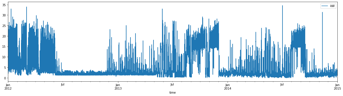
Our dataset consists of hourly kW readings for multiple buildings:

df_elec.head()

	group	time	kW
0	MT_001	2012-01-01 00:00:00	3.172589
1	MT_001	2012-01-01 01:00:00	4.124365
2	MT_001	2012-01-01 02:00:00	4.758883
3	MT_001	2012-01-01 03:00:00	4.441624
4	MT_001	2012-01-01 04:00:00	4.758883

Electricity-demand data can be challenging because of its complexity. In traditional forecasting applications, we divide our model into siloed processes that each contribute to separate behaviors of the time-series. For example:

• Hour-in-day effects

• Day-in-week effects

• Season-in-year effects

• Weather effects

However, with electricity data, it’s limiting to model these separately, because these effects all interact: the impact of hour-in-day depends on the day-of-week, the impact of the day-of-week depends on the season of the year, etc.

We can plot some examples to get an initial glance at this complexity.

df_elec.query("group=='MT_001'").plot('time', 'kW', figsize=(20, 5))

<AxesSubplot:xlabel='time'>

Some groups have data that isn’t really appropriate for modeling – for example, exhibiting near-zero variation:

df_elec.query("group=='MT_003'").plot('time', 'kW', figsize=(20, 5))

<AxesSubplot:xlabel='time'>

For some rudimentary cleaning, we’ll remove these kinds of regions of ‘flatness’. For simplicity we’ll just drop buildings that are flat in this way for a non-trivial amount of time.

# calculate rolling std-dev:
df_elec['roll_std'] = df_elec.groupby('group')['kW'].rolling(48).std().reset_index(0, drop=True)
# set to missing when it's low
df_elec.loc[df_elec.pop('roll_std') < .25, 'kW'] = float('nan')
# drop groups with nontrivial amount of missings (for simplicity)
group_missingness = df_elec.assign(missing=lambda df: df['kW'].isnull()).groupby('group')['missing'].mean()
df_elec = df_elec.loc[df_elec['group'].map(group_missingness) < .01, :].reset_index(drop=True)

We’ll split the data at mid-2013. For half the groups, the holdout will be used as validation data; for the other half, it will be used as test data.

SPLIT_DT = np.datetime64('2013-06-01')
df_elec['_use_holdout_as_test'] = (df_elec['group'].str.replace('MT_', '').astype('int') % 2) == 0
df_elec['dataset'] = 'train'
df_elec.loc[(df_elec['time'] >= SPLIT_DT) & df_elec['_use_holdout_as_test'], 'dataset'] = 'test'
df_elec.loc[(df_elec['time'] >= SPLIT_DT) & ~df_elec.pop('_use_holdout_as_test'), 'dataset'] = 'val'

Finally, drop groups without enough data:

df_group_summary = df_elec. \
    groupby(['group','dataset']) \
    ['time'].agg(['min', 'max']). \
    reset_index(). \
    assign(history_len=lambda df: (df['max'] - df['min']).dt.days)

all_groups = set(df_group_summary['group'])
train_groups = sorted(df_group_summary.query("(dataset=='train') & (history_len >= 365)")['group'])
df_elec = df_elec.loc[df_elec['group'].isin(train_groups), :].reset_index(drop=True)

Let’s pick an example group to focus on, for demonstrative purposes:

example_group = 'MT_358'

A Standard Forecasting Approach

Attempt 1

First, let’s try a standard exponential-smoothing algorithm on one of the series. This intentionally doesn’t leverage torchcast’s ability to train on batches of series, so is quite slow, but will help us have a base case to improve on.

from torchcast.process import LocalTrend, Season

es = ExpSmoother(
    measures=['kW_sqrt_c'],
    processes=[
        # seasonal processes:
        Season(id='day_in_week', period=24 * 7, dt_unit='h', K=3, fixed=True),
        Season(id='day_in_year', period=24 * 365.25, dt_unit='h', K=8, fixed=True),
        Season(id='hour_in_day', period=24, dt_unit='h', K=8, fixed=True),
        # long-running trend:
        LocalTrend(id='trend'),
    ]
)

# transform and center:
df_elec['kW_sqrt'] = np.sqrt(df_elec['kW'])
group_means = df_elec.query("dataset=='train'").groupby('group')['kW_sqrt'].mean().to_dict()
df_elec['kW_sqrt_c'] = df_elec['kW_sqrt'] - df_elec['group'].map(group_means)

# build our dataset
train_example = TimeSeriesDataset.from_dataframe(
    df_elec.query("group == @example_group").query("dataset == 'train'"),
    group_colname='group',
    time_colname='time',
    dt_unit='h',
    measure_colnames=['kW_sqrt_c'],
)
train_example

TimeSeriesDataset(sizes=[torch.Size([1, 12408, 1])], measures=(('kW_sqrt_c',),))

try:
    es.load_state_dict(torch.load(os.path.join(BASE_DIR, f"es_{example_group}.pt")))
except FileNotFoundError:
    es.fit(
        train_example.tensors[0],
        start_offsets=train_example.start_datetimes,
    )
    torch.save(es.state_dict(), os.path.join(BASE_DIR, f"es_{example_group}.pt"))

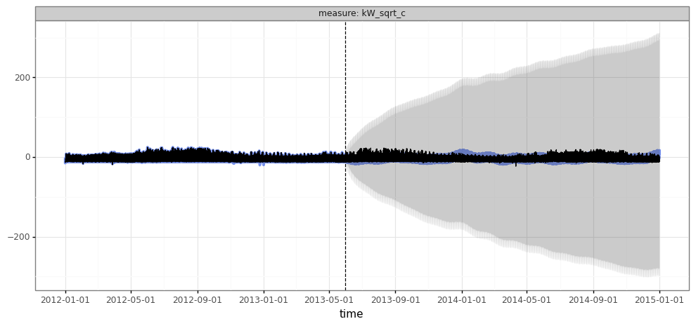
How does this standard model perform? Plotting the forecasts vs. actual suggests serious issues:

from torchcast.state_space import Predictions

@torch.no_grad()
def make_forecast_df(
        model: ExpSmoother,
        df_trainval: pd.DataFrame,
        **kwargs) -> pd.DataFrame:
    batch = TimeSeriesDataset.from_dataframe(
        df_trainval,
        group_colname='group',
        time_colname='time',
        dt_unit='h',
        measure_colnames=['kW_sqrt_c'],
    )
    # subset data to just train:
    train_y = batch.train_val_split(dt=SPLIT_DT)[0].tensors[0]
    # generate forecast:
    pred = model(
        train_y,
        start_offsets=batch.start_times,
        out_timesteps=batch.tensors[0].shape[1],  # outputs times that include validation period,
        **kwargs
    )
    # convert to df:
    return pred.to_dataframe(batch).query("actual.notnull()", engine='python').reset_index(drop=True)


def plot_forecasts(df: pd.DataFrame, **kwargs):
    kwargs['split_dt'] = kwargs.get('split_dt', SPLIT_DT)
    return Predictions.plot(df, **kwargs)


df_forecast_ex = make_forecast_df(model=es, df_trainval=df_elec.query("group == @example_group"))

plot_forecasts(df_forecast_ex)

<ggplot: (8758008614897)>

The most obvious issue here is the discrepancy between the predictions on the training data (which look sane) and the validation data (which look insane). This isn’t overfitting, but instead the difference between one-step-ahead predictions vs. long-range forecasts. One possibility for why the model does so poorly on the latter is that it wasn’t actually trained to generate these predictions: the standard approach has us train on one-step-ahead predictions.

Attempt 2

Let’s see if we can improve on this. We’ll leave the model unchanged but make two changes:

• Use the n_step argument to train our model on one-week ahead forecasts, instead of one step (i.e. hour) ahead. This improves the efficiency of training by encouraging the model to ‘care about’ longer range forecasts vs. over-focusing on the easier problem of forecasting the next hour.

• Split our single series into multiple groups. This is helpful to speed up training, since pytorch has a non-trivial overhead for separate tensors – i.e., it scales well with an increasing batch-size (fewer, but bigger, tensors), but poorly with an increasing time-series length (smaller, but more, tensors).

# for efficiency of training, we split this single group into multiple groups
df_elec['gyq'] = \
    df_elec['group'] + ":" + \
    df_elec['time'].dt.year.astype('str') + "_" + \
    df_elec['time'].dt.quarter.astype('str')

# since TimeSeriesDataset pads short series, drop incomplete groups:
df_elec.loc[df_elec.groupby('gyq')['kW_sqrt'].transform('count') < 2160, 'gyq'] = float('nan')

train_example_2 = TimeSeriesDataset.from_dataframe(
    df_elec.query("group == @example_group").query("dataset == 'train'"),
    group_colname='gyq',
    time_colname='time',
    dt_unit='h',
    measure_colnames=['kW_sqrt_c'],
)

try:
    es.load_state_dict(torch.load(os.path.join(BASE_DIR, f"es_{example_group}_2.pt")))
except FileNotFoundError:
    es.fit(
        train_example_2.tensors[0],
        start_offsets=train_example_2.start_datetimes,
        n_step=int(24 * 7.5),
        every_step=False
    )
    torch.save(es.state_dict(), os.path.join(BASE_DIR, f"es_{example_group}_2.pt"))

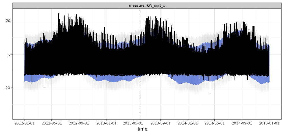
df_forecast_ex2 = make_forecast_df(model=es, df_trainval=df_elec.query("group == @example_group"))
plot_forecasts(df_forecast_ex2)

<ggplot: (8758008589117)>

Seems like a massive improvement… Unfortunately, with hourly data, visualizing long-range forecasts in this way isn’t very illuminating: it’s just really hard to see the data!

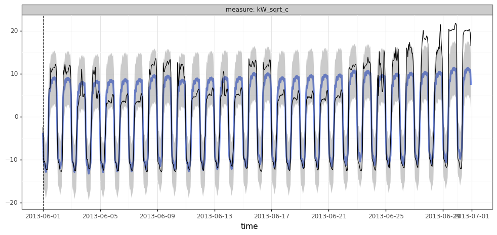
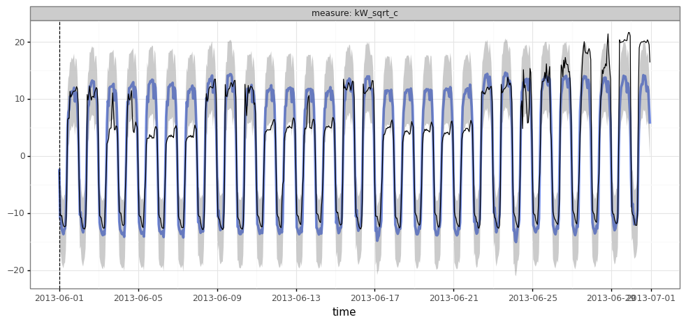
We can try zooming in:

plot_forecasts(df_forecast_ex2.query("time.dt.year==2013 & time.dt.month==6"))

<ggplot: (8758008110329)>

This is better for actually seeing the data, but ideally we’d still like to get a view of the long range.

Let’s instead try splitting it into weekdays vs. weekends and daytimes vs. nightimes:

def plot_2x2(df: pd.DataFrame,
             time_colname: str = 'time',
             pred_colname: str = 'mean',
             actual_colname: str = 'actual',
             day_hours: tuple = (14, 15, 16, 17, 18),
             night_hours: tuple = (2, 3, 4, 5, 6),
             **kwargs):
    """
    Plot predicted vs. actual for a single group, splitting into 2x2 facets of weekday/end * day/night.
    """
    assert pred_colname in df.columns
    assert actual_colname in df.columns
    if 'group' in df.columns:
        assert df['group'].nunique() == 1

    df_split = df.loc[df[time_colname].dt.hour.isin(day_hours) | df[time_colname].dt.hour.isin(night_hours), :]. \
        assign(weekend=lambda df: df[time_colname].dt.weekday.isin([5, 6]).astype('int'),
               night=lambda df: (df[time_colname].dt.hour.isin(night_hours)).astype('int'),
               date=lambda df: df[time_colname].astype('datetime64[D]')). \
        groupby(['date', 'weekend', 'night']). \
        agg(forecast=(pred_colname, 'mean'), actual=(actual_colname, 'mean')). \
        reset_index()

    kwargs['subplot_kw'] = kwargs.get('subplot_kw', {})
    if 'ylim' not in kwargs['subplot_kw']:
        kwargs['subplot_kw']['ylim'] = (df_split['actual'].min(), df_split['actual'].max())

    _, axes = plt.subplots(ncols=2, nrows=2, figsize=(15, 10), **kwargs)
    for (wknd, night), df in df_split.groupby(['weekend', 'night']):
        df.plot('date', 'actual', ax=axes[wknd, night], linewidth=.5, color='black')
        df.plot('date', 'forecast', ax=axes[wknd, night], alpha=.75, color='red')
        axes[wknd, night].axvline(x=SPLIT_DT, color='black', ls='dashed')
        axes[wknd, night].set_title("{}, {}".format('Weekend' if wknd else 'Weekday', 'Night' if night else 'Day'))
    plt.tight_layout()


plot_2x2(df_forecast_ex2)

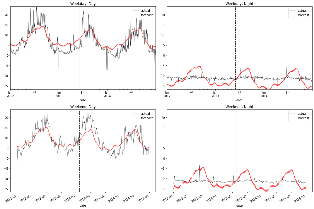
Viewing the forecasts in this way helps us see a lingering serious issue: the annual seasonal pattern is very different for daytimes and nighttimes, but the model isn’t capturing that.

The limitation is inherent to the model: it only allows for a single seasonal pattern, rather than a separate one for different times of the day and days of the week.

Incorporating a Neural Network

If the problem is that our time-series model isn’t allowing for interactions among the components of our time-series model, then a natural approach to allowing for these interactions is a neural network.

To make this work, we likely don’t want build a model of a single series. Instead, we want to learn across multiple series, so that our network can build representations of patterns that are shared across multiple buildings.

First, we’ll use torchcast.utils.add_season_features to add dummy features that capture the annual, weekly, and daily seasonal patterns:

from torchcast.utils import add_season_features

df_elec = df_elec. \
    pipe(add_season_features, K=3, period='weekly'). \
    pipe(add_season_features, K=8, period='yearly'). \
    pipe(add_season_features, K=10, period='daily')

season_cols = \
    df_elec.columns[df_elec.columns.str.endswith('_sin') | df_elec.columns.str.endswith('_cos')].tolist()

Since we’re working with more data, we’ll need to use a dataloader (torchcast provies TimeSeriesDataLoader):

def make_dataloader(type_: str,
                    batch_size: int,
                    group_colname: str = 'group',
                    **kwargs) -> TimeSeriesDataLoader:
    assert type_ in {'train', 'val', 'all'}
    data = df_elec if type_ == 'all' else df_elec.query(f"dataset == '{type_}'")
    return TimeSeriesDataLoader.from_dataframe(
        data,
        group_colname=group_colname,
        X_colnames=season_cols,
        y_colnames=['kW_sqrt_c'],
        time_colname='time',
        dt_unit='h',
        **kwargs,
        batch_size=batch_size
    )

Intro

Our goal is to make a ‘hybrid’ model that combines the traditional approach (here, exponential smoothing) with a neural network.

Specifying this is straightforward. The LinearModel provides a catch-all for any way of passing arbitrary inputs to our model. For example, if we had weather data – temperature, humidity, wind-speed – we might add a process like:

LinearModel(id='weather', predictors=['temp','rhumidity','windspeed'])

And our time-series model would learn how each of these impacts our series(es).

Here we are using LinearModel a little differently: rather than it taking as input predictors, it will take as input the output of a neural-network, which itself will take predictors (the calendar-features we just defined).

from torchcast.process import LinearModel, LocalLevel

es_nn = ExpSmoother(
    measures=['kW_sqrt_c'],
    processes=[
        # trend:
        LocalTrend(id='trend'),
        # static seasonality:
        LinearModel(id='season', predictors=['nn_output']),
        # local deviations from typical behavior:
        LocalLevel(id='local_level', decay=True),
        Season(id='local_hour_in_day', period=24, dt_unit='h', K=6, decay=True),
    ]
)

Pre-Training

Now all we have to do is prepare a neural network that takes our annual/weekly/hourly features as inputs and produces predictions. We could simply define a network, pass its outputs to es_nn, and train the whole thing end-to-end. In practice, however, it’s more efficient to first ‘pre-train’ our network, since it requires many more iterations than the ExpSmoother (and is faster per-iteration).

To keep things (relatively) concise, we’ll use PyTorch Lightning.

Since we’ll use this again later, we first make an abstract class that works on any model with a TimeSeriesDataset input:

# GPU will be useful if we have one:
maybe_cuda = torch.device('cuda' if torch.cuda.is_available() else 'cpu')
maybe_cuda

device(type='cpu')

from pytorch_lightning import LightningModule, Trainer
from pytorch_lightning.callbacks.early_stopping import EarlyStopping
from pytorch_lightning.loggers import CSVLogger
from torch_optimizer import Adahessian



class TimeSeriesLightningModule(LightningModule):
    def __init__(self, module: torch.nn.Module):
        super().__init__()
        self._module = module

    def _step(self, batch: TimeSeriesDataset, batch_idx: int, **kwargs) -> torch.Tensor:
        batch = batch.to(maybe_cuda)
        pred = self(batch, **kwargs)
        return self._get_loss(pred, batch.tensors[0])

    def training_step(self, batch: TimeSeriesDataset, batch_idx: int, **kwargs) -> torch.Tensor:
        loss = self._step(batch, batch_idx=batch_idx, **kwargs)
        self.log("step_train_loss", loss, on_step=True, on_epoch=False)
        self.log("epoch_train_loss", loss, on_step=False, on_epoch=True)
        return loss

    @torch.no_grad()
    def validation_step(self, batch: TimeSeriesDataset, batch_idx: int, **kwargs) -> torch.Tensor:
        loss = self._step(batch, batch_idx=batch_idx, **kwargs)
        self.log("step_val_loss", loss, on_step=True, on_epoch=False)
        self.log("epoch_val_loss", loss, on_step=False, on_epoch=True)
        return loss

    def _get_loss(self, predicted, actual) -> torch.Tensor:
        raise NotImplementedError

    def forward(self, batch: TimeSeriesDataset, **kwargs) -> torch.Tensor:
        raise NotImplementedError

Now we’ll make a class that’s more specific to the current task.

There are a variety of ways we could do this. Here, we’re approaching it by combining two kinds of networks:

1. A multi-layer network takes the calendar-features and produces multiple outputs.

2. An embedding network takes the groups and produces an embedding of the same dim.

To generate a prediction, we multiply the two. We can almost think of this like the first network is learning dimensionality reduction – reducing the dozens of calendar-features (and their hundreds of interactions) into an efficient low-dimensional representation – and the second network is learning the group-specific coefficients for these derived features.

names_to_idx = {nm: int(nm.replace('MT_','')) - 1 for nm in df_elec['group'].unique()}

class CalendarFeatureNN(TimeSeriesLightningModule):
    def __init__(self, module: torch.nn.Module):
        super().__init__(module=module)
        with torch.no_grad():
            self._module.emb_nn.weight *= .1

    def _get_loss(self, predicted, actual) -> torch.Tensor:
        is_valid = ~torch.isnan(actual)
        sq_err = (actual[is_valid] - predicted[is_valid]) ** 2
        return sq_err.mean()

    def backward(self,
                loss: torch.Tensor,
                optimizer: torch.optim.Optimizer,
                optimizer_idx: int,
                *args,
                **kwargs):
                return super().backward(loss, optimizer, optimizer_idx, create_graph=True)

    def forward(self, batch: TimeSeriesDataset, **kwargs) -> torch.Tensor:
        y, X = batch.tensors
        group_names = [gn.split(":")[0] for gn in batch.group_names]
        group_ids = [names_to_idx[gn] for gn in group_names]

        # use NNs to get latent features and group-specific coefs on those features:
        coefs = self._module.emb_nn(torch.tensor(group_ids, device=maybe_cuda))
        feats = self._module.features_nn(X)

        # multiply features by coefs (as in a linear-model)
        # NOTE: no bias term -- assumes centered y
        pred = (coefs.unsqueeze(1) * feats).sum(-1, keepdim=True)

        return pred

    def configure_optimizers(self) -> torch.optim.Optimizer:
        pars = [p for p in self.parameters() if p.requires_grad]
        return Adahessian(pars, lr=.15)

cal_features_num_latent_dim = 25

calendar_feature_nn = CalendarFeatureNN(
    torch.nn.ModuleDict({'features_nn':
        torch.nn.Sequential(
            torch.nn.Linear(len(season_cols), 48),
            torch.nn.Tanh(),
            torch.nn.Linear(48, 48),
            torch.nn.Tanh(),
            torch.nn.Linear(48, cal_features_num_latent_dim)
        )
        , 'emb_nn':
            torch.nn.Embedding(
                num_embeddings=370,
                embedding_dim=cal_features_num_latent_dim
            )
    })
).to(maybe_cuda)

try:
    calendar_feature_nn.load_state_dict(torch.load(
        os.path.join(BASE_DIR, f"calendar_feature_nn{cal_features_num_latent_dim}.pt")
    ))
except FileNotFoundError:
    Trainer(
        gpus=int(str(maybe_cuda) == 'cuda'),
        logger=CSVLogger(BASE_DIR, f'calendar_feature_nn{cal_features_num_latent_dim}'),
        log_every_n_steps=1,
        min_epochs=100,
        callbacks=[EarlyStopping(monitor="epoch_val_loss", patience=10, min_delta=.0001, verbose=False)]
    ).fit(calendar_feature_nn, make_dataloader('train', batch_size=45), make_dataloader('val', batch_size=55))
    calendar_feature_nn.trainer = None
    torch.save(
        calendar_feature_nn.state_dict(), os.path.join(BASE_DIR, f"calendar_feature_nn{cal_features_num_latent_dim}.pt")
    )

Evaluation

Let’s return to our example group. This neural-network only takes calendar-features as input, so it’s unable to incorporate trends or autocorrelation. Still, we can get a glimpse of whether it’s able to handle the interacting seasonalities problem.

calendar_feature_nn.to(maybe_cuda)

eval_example = TimeSeriesDataset.from_dataframe(
    df_elec[df_elec['group'] == example_group],
    group_colname='group',
    X_colnames=season_cols,
    y_colnames=['kW_sqrt_c'],
    time_colname='time',
    dt_unit='h',
).to(maybe_cuda)

with torch.no_grad():
    df_cal_nn_example = TimeSeriesDataset.tensor_to_dataframe(
        calendar_feature_nn(eval_example),
        times=eval_example.times(),
        group_names=eval_example.group_names,
        time_colname='time', group_colname='group',
        measures=['predicted_sqrt']
    ).merge(df_elec[df_elec['group'] == example_group], how='left')

plot_2x2(df_cal_nn_example, actual_colname='kW_sqrt_c', pred_colname='predicted_sqrt')

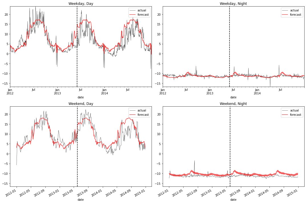
We can see that the network correctly captures the varying seasonal patterns.

The Hybrid Model

Now we’re reading to plug our network into our ExpSmoother.

# freeze the "features" while keeping the per-building embeddings unfrozen:
[p.requires_grad_(False) for p in calendar_feature_nn._module.features_nn.parameters()]

# pytorch has the handy feature that we can set calendar_feature_nn to be a child of es_nn
# by adding it as an attribute; among other things this means that calendar_feature_nn's params
# will be included in the state-dict:
es_nn.calendar_feature_nn = copy.deepcopy(calendar_feature_nn)

One More Thing: Predict Variance

One last complexity we’re going to add:

Our exponential-smoothing model has the nice property that it doesn’t just generate point-predictions, but also prediction intervals (the gray bands we see when we use plot_forecasts()).

While we aren’t using these centrally in the current example, we’re still going to be responsible forecasters and try to make these generally well-calibrated. When predicting multiple series where the values can vary greatly – as we are here, with multiple buildings whose kW usage can vary based on the building’s size and other factors – we would not generally expect the variance to be the same across series. This can be mitigated somewhat by centering/scaling the series, but this is limited (e.g. scaling a series by its std-deviation confounds variation due to inherent noise in the series and variation due to annual seasonality). A better approach is to predict the variance.

Here we will set up our ExponentialSmoother to predict the variance. Ther are a variety of ways we could do this (e.g. an embedding to allow each series to have a separate variance; or even support time-varying variances), but here we will take a relatively simple approach of predicting based on means/std-dev.

group_resid_devs = df_elec. \
    query("dataset=='train'"). \
    assign(_diff=lambda df: df.groupby('group')['kW_sqrt'].diff()). \
    pipe(lambda df: df.groupby('group')['_diff'].std().to_dict())


def make_group_features_mat(group_names: Sequence[str]) -> torch.Tensor:
    means = torch.as_tensor([group_means[gn] for gn in group_names], device=maybe_cuda)
    devs = torch.as_tensor([group_resid_devs[gn] for gn in group_names], device=maybe_cuda)
    cvs = devs / means
    return torch.stack([means, devs, cvs], 1).log()

make_group_features_mat([example_group])

tensor([[ 3.2962,  1.3264, -1.9697]])

from torchcast.covariance import Covariance

es_nn.measure_covariance = Covariance.from_measures(['kW_sqrt_c'], predict_variance=True)

es_nn.measure_var_nn = torch.nn.Sequential(
    torch.nn.Linear(3,1),
    torch.nn.Softplus()
)

Training

We’ll again create a lightning class to help with training:

class HybridForecaster(TimeSeriesLightningModule):
    def _get_loss(self, predicted, actual) -> torch.Tensor:
        return -predicted.log_prob(actual).mean()

    def _step(self, batch: TimeSeriesDataset, batch_idx: int, **kwargs) -> torch.Tensor:
        return super()._step(batch=batch, batch_idx=batch_idx, n_step=int(24 * 15), every_step=False, **kwargs)

    def forward(self, batch: TimeSeriesDataset, **kwargs) -> torch.Tensor:
        y, X = batch.tensors
        group_names = [gn.split(":")[0] for gn in batch.group_names]
        mvar_X = make_group_features_mat(group_names)

        return self._module(
            y,
            season__X=self._module.calendar_feature_nn(batch),
            measure_var_multi=self._module.measure_var_nn(mvar_X),
            start_offsets=batch.start_offsets,
            **kwargs
        )

    def backward(self, *args, **kwargs):
        return super().backward(*args, **kwargs, create_graph=True)

    def configure_optimizers(self) -> torch.optim.Optimizer:
        return Adahessian([p for p in self.parameters() if p.requires_grad], lr=.10)

es_nn_lightning = HybridForecaster(es_nn)

try:
    es_nn.load_state_dict(torch.load(os.path.join(BASE_DIR, f"es_nn{cal_features_num_latent_dim}.pt")))
except FileNotFoundError:
    Trainer(
        gpus=int(str(maybe_cuda) == 'cuda'),
        logger=CSVLogger(BASE_DIR, f'es_nn{cal_features_num_latent_dim}', flush_logs_every_n_steps=1),
        log_every_n_steps=1,
        min_epochs=10,
        callbacks=[EarlyStopping(monitor="epoch_val_loss", patience=10, min_delta=0.001, verbose=True)]
    ).fit(es_nn_lightning,
          make_dataloader('train', batch_size=144, group_colname='gyq', shuffle=True),
          make_dataloader('val', batch_size=55)
          )
    torch.save(es_nn.state_dict(), os.path.join(BASE_DIR, f"es_nn{cal_features_num_latent_dim}.pt"))

Evaluation

Reviewing the same example-building from before, we see the forecasts are more closely hewing to the actual seasonal structure for each time of day/week. Instead of the forecasts in each panel being essentially identical, each differs in shape.

plot_forecasts(df_forecast_nn.query("group==@example_group & time.dt.year==2013 & time.dt.month==6"))

<ggplot: (8758005274605)>

plot_2x2(df_forecast_nn.query("group==@example_group"))

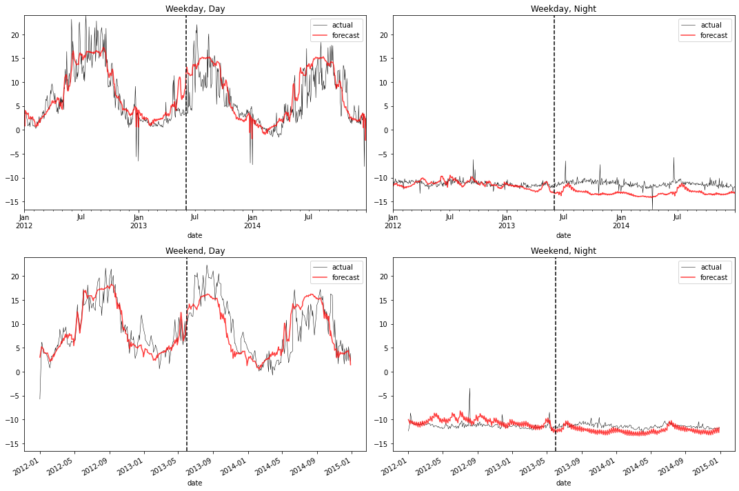
Let’s confirm quantitatively that the 2nd model does indeed substantially reduce forecast error, relative to the ‘standard’ model:

def inverse_transform(df: pd.DataFrame) -> pd.DataFrame:
    df = df.copy()
    for col in ['mean', 'lower', 'upper', 'actual']:
        df[col] = df[col] + df['group'].map(group_means)
        df[col] = df[col].clip(lower=0) ** 2
    return df

df_nn_err = df_forecast_nn. \
    pipe(inverse_transform).\
    assign(error=lambda df: (df['mean'] - df['actual']).abs(),
           validation=lambda df: df['time'] > SPLIT_DT). \
    groupby(['group', 'validation']). \
    agg(error=('error', 'mean')). \
    reset_index()

df_forecast_ex2. \
    pipe(inverse_transform).\
    assign(error=lambda df: (df['mean'] - df['actual']).abs(),
           validation=lambda df: df['time'] > SPLIT_DT). \
    groupby(['group', 'validation']). \
    agg(error=('error', 'mean')). \
    reset_index(). \
    merge(df_nn_err, on=['group', 'validation'], suffixes=('_es', '_es_nn'))

	group	validation	error_es	error_es_nn
0	MT_358	False	142.691729	102.412429
1	MT_358	True	156.775703	142.027575